
Suppose we have an industrial robot arm with six joints. Even a small turn of one joint moves the whole arm behind it, and the hand at the tip ends up somewhere entirely different. To compute this chain of motion, we first need a fixed way of writing how each joint and link is shaped. If everyone picks their own frame of reference, the same robot yields different equations. The agreement that neatly captures these relations with just four numbers per joint—that is the ‘Denavit-Hartenberg Convention.’
Put simply, the Denavit-Hartenberg convention means ‘a method of attaching coordinate frames to each joint of a serial robot arm by a fixed rule, and expressing the relation between two neighboring frames with four parameters.’ In 1955 Jacques Denavit (Jacques Denavit) and Richard Hartenberg (Richard Hartenberg) first proposed it to standardize coordinate frames for mechanical linkages. It is often shortened to DH convention or DH parameters, and it is still among the first tools taught in robotics textbooks.
In this piece we will look, in order, at why this convention was needed, what each of the four numbers means, how chaining the numbers yields the end-effector position, and how the classical and modified forms came to diverge.
The agreement that writes a robot arm with four numbers
Why did the Denavit-Hartenberg convention arise?

A robot arm is a chain of rigid links joined by joints. To know where the end effector is, you must account for every link’s length and orientation and how far each joint has turned. The catch is that describing an object’s position and orientation in space originally takes six values.
(1) Coordinate frames that differed from person to person
Before the convention settled in, each researcher attached axes differently. Even analyzing the same machine produced differently shaped equations, making results hard to compare or review.
(2) The 1955 proposal
Denavit and Hartenberg presented a matrix-based kinematic notation in a paper in the ASME Journal of Applied Mechanics. The key idea was that once rules for attaching axes are fixed, the relation between neighboring links can be reduced from six values to four.
(3) The period when it crossed into robotics
At first it was a method for general mechanical linkages. In 1981 Richard Paul (Richard Paul) put the convention to full use for robot-arm analysis in a robot manipulators textbook, and it took hold as a standard tool in robotics.
The four numbers attached to each joint
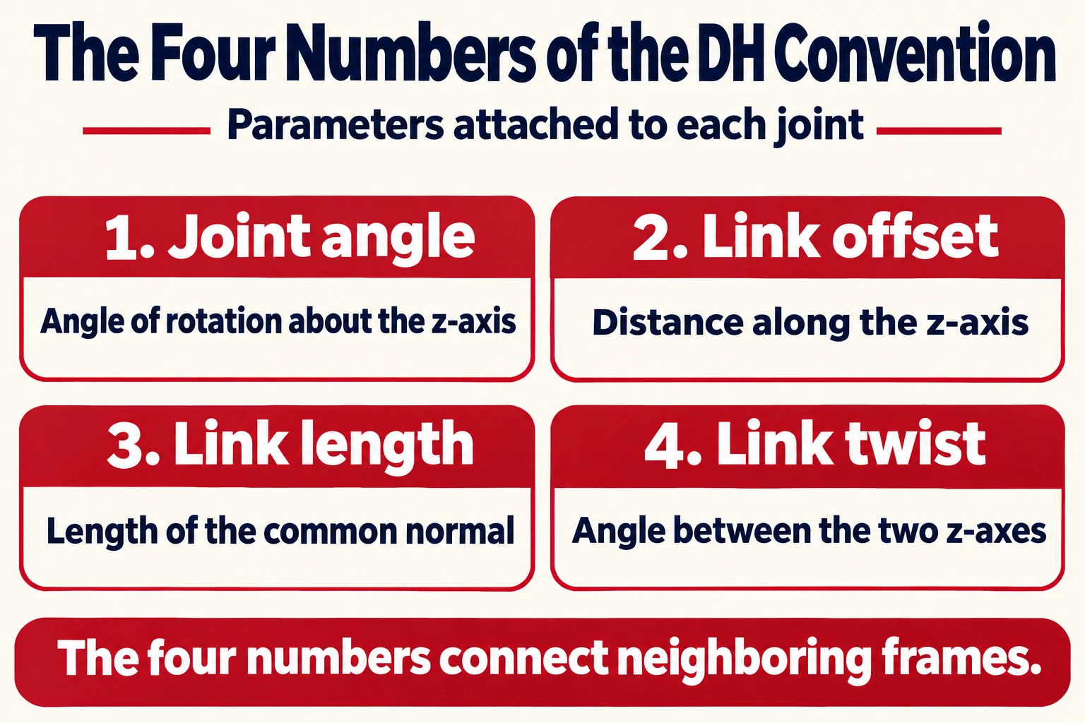
The rule is surprisingly simple. Take each joint’s axis of rotation or sliding direction as the z-axis, and take the common normal—the line perpendicular to both neighboring joint axes—as the x-axis. Once the axes are aligned this way, only four values remain to go from one frame to the next.
- Joint Angle (Joint Angle): The angle by which the x-axis has rotated about the previous z-axis.
- Link Offset (Link Offset): The distance along the previous z-axis to the next common normal.
- Link Length (Link Length): The length of the common normal between the two joint axes.
- Link Twist (Link Twist): The angle by which the two z-axes are skewed about the common normal.
For a revolute joint the joint angle changes with the motor while the other three stay fixed by the machine’s geometry. For a prismatic joint, conversely, the link offset is the varying value. In the end each joint carries one moving number and three numbers that fix the shape.
Chaining the table to find the end effector

Writing the four numbers in joint order produces a simple table—one row per joint—that holds the whole robot arm. With that table alone, computing the end-effector position becomes a mechanical procedure.
(1) Transforms that step one cell at a time
The numbers in each row become one coordinate transform: four steps of motion that rotate and translate along z, then translate and rotate along x. This transform is arranged as a 4×4 matrix that holds rotation and position together.
(2) Multiply in order and you are done
Multiplying in sequence the matrices from base to first joint, first to second, and so on yields a single matrix relating base to end effector. Plug in only the joint angles and the end-effector position and orientation are computed at once. That is the basic frame of forward kinematics.
(3) A starting point for other calculations
The same table is used as-is for inverse kinematics—recovering joint angles from a desired end-effector pose—and for dynamics that handle velocity and force. That is also why many robot simulation programs take this table as input.
Classical and modified: two branches of the agreement
As widely used as it is, there is confusion too. Two methods share the same name. That is why, when you open a textbook or a program, you should first check which side it follows.
(1) Classical convention
In the original method, each link’s coordinate frame is attached at the joint at the far end of that link. Many textbooks and open materials explain from this baseline.
(2) Modified convention
Used in texts such as John Craig’s (John Craig) Introduction to Robotics (Introduction to Robotics), this form attaches frames at the joint at the start of the link and also changes the transform order. Parameter names look similar but the slots differ, so mixing the two yields wrong results.
(3) Limits and alternatives
When two neighboring joint axes are nearly parallel, the common normal’s position is ill-defined and small errors swing the values widely. Fields that need precise calibration have therefore also studied other representations. Even so, because it is simple and easy to follow by hand, it remains the first method taught.
Writing even a complex-looking robot arm carefully with four numbers per joint—that is the first step in understanding the Denavit-Hartenberg convention.