The data in the real world we live in are never neatly organized. Some data are skewed to one side, some have multiple peaks, and others are scattered irregularly without any pattern.
Yet statisticians accurately estimate the characteristics of the whole even from such disorderly data. When investigating the average height of all adults in South Korea or support rates in a nationwide election, what is the secret to predicting results with high accuracy without surveying every person?
At the heart of this is the Central Limit Theorem (CLT), regarded as one of the most beautiful and powerful theorems in statistics.

In statistics, the entire group we really want to learn about is called the population (Population), and a group drawn from part of the population because of practical constraints is called a sample (Sample).
It can be difficult to know in advance whether the population follows a normal distribution (a symmetric, bell-shaped distribution). Inference is possible without knowing its exact distribution, but the sampling design and distributional conditions required by the chosen method must be checked.
The basic central limit theorem concerns averages of independent, identically distributed observations. If the population has a finite mean and a positive, finite variance, the distribution of the standardized sample mean approaches the standard normal distribution as the sample size increases.
The Mechanism of the Central Limit Theorem
The Mathematical Definition of the Central Limit Theorem
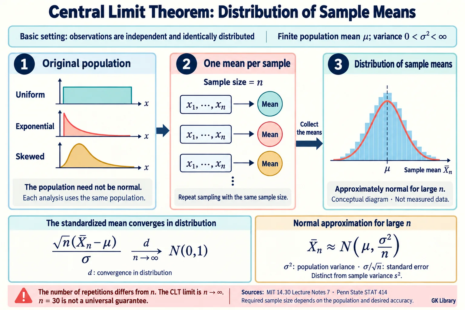
The central limit theorem can be expressed academically as follows.
[Definition]
Let X̄ₙ be the mean of independent, identically distributed observations X₁, …, Xₙ, with population mean μ and variance σ² (0 < σ² < ∞). As n → ∞, √n(X̄ₙ − μ)/σ converges in distribution to the standard normal distribution N(0, 1). Thus, for sufficiently large n, the distribution of X̄ₙ can be approximated by N(μ, σ²/n). Here σ² is the population variance, distinct from the sample variance s². The required sample size depends on features such as skewness and tails, so n = 30 is not a universal guarantee of an adequate approximation.
There are 3 key points to keep in mind here.
- The theorem applies to uniform, exponential, and asymmetric populations when independence, identical distributions, a finite mean, and a positive, finite variance hold.
- The normal approximation concerns the distribution of sample means, rather than the original observations. To understand this distribution, repeatedly draw samples of a fixed size n in the same way and calculate one mean from each sample.
- Under these conditions, the standard error of the sample mean is σ/√n. If the population standard deviation σ is unknown, it can be estimated by s/√n using the sample standard deviation s.
An Intuitive Example to Aid Understanding: Rolling Dice
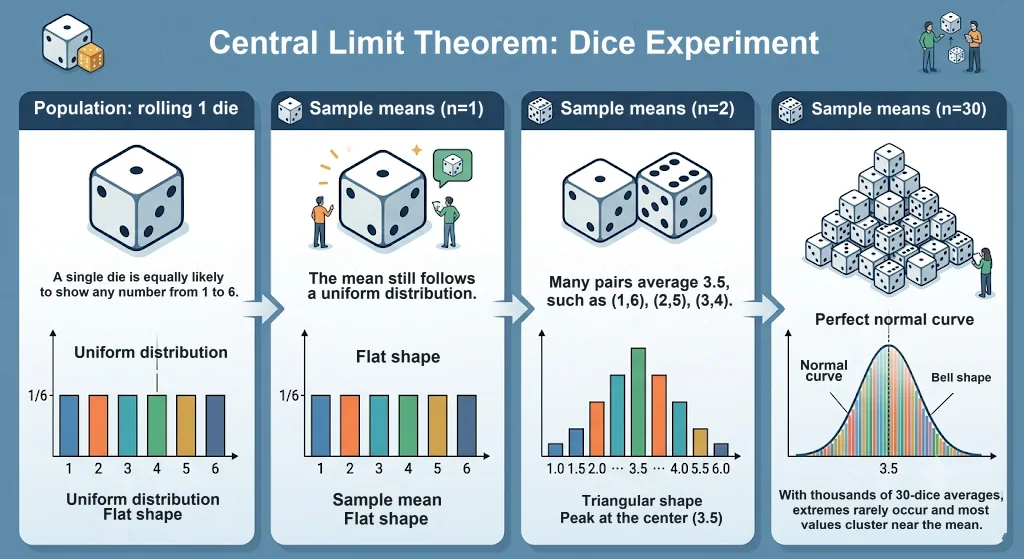
If the concept of the central limit theorem feels difficult to grasp, let us consider the simplest experiment of rolling dice.
When 1 die is rolled, each face from 1 to 6 has the same probability of 1 in 6. When plotted on a graph, this probability distribution takes the form of a flat uniform distribution (Uniform Distribution). It is far from bell-shaped.
Now let us increase the number of dice rolls (the sample size n) and calculate the "mean" of the face values.
1 die (n=1): The possible means are 1, 2, 3, 4, 5, and 6, and every face has the same probability. (A flat, straight-line shape)
Mean of 2 dice (n=2): For the mean of the two dice to be 1, the only possible outcome is (1, 1), whereas a mean of 3.5 can arise from many combinations, such as (1, 6), (2, 5), and (3, 4). The graph becomes triangular, rising at the center (3.5) and falling at both ends.
Mean of 30 dice (n=30): If the process of rolling 30 dice and calculating their mean is repeated thousands of times, extreme values (a mean of 1 or 6) virtually never occur, and most values cluster densely around 3.5.
The histogram of these sample means will generally be approximately bell-shaped. A finite experiment does not produce a perfect normal curve, and dice averages still take discrete values. This example assumes fair dice and independent rolls.
Key Implications of the Central Limit Theorem

[Implication 1] Distributional Autonomy
Under the conditions stated above, a normal approximation for the sample mean can be used even when the population is asymmetric or skewed. The sample size needed for the approximation depends on the distribution.
[Implication 2] Increased Estimation Accuracy
Under these conditions, increasing n reduces the standard error, concentrating the distribution of sample means more closely around the population mean. This does not mean that each individual sample mean necessarily gets closer.
[Implication 3] Using Standardization Techniques
When the conditions hold and the normal approximation is sufficiently accurate, the approximate distribution of the standardized sample mean can be used to calculate confidence intervals and p-values. When σ is unknown, uncertainty in its estimation must also be considered.
Applications in Everyday Life and Business

The central limit theorem extends beyond a mere academic theory and serves as a key tool in countless areas of modern society.
Election Opinion Polls by Broadcasters
Surveying the entire national electorate, numbering 4 times ten million people, is impossible in terms of cost and time. Polling organizations typically draw samples of 1,000 to 2,000 people to survey support rates. With an appropriate probability sample and adequate approximation conditions, the sampling distribution of a proportion can be approximated by a normal distribution to calculate a margin of error. For example, assuming a simple random sample of n = 1,000, a proportion of 50%, and ignoring the finite-population correction, the approximate 95% margin of error is ±3.1 percentage points. This does not include all sources of error, such as nonresponse or measurement error.
Quality Control in Factory Manufacturing (6 Sigma)
Factories producing semiconductors or beverages cannot measure the weight and thickness of every product manufactured each hour. They continuously calculate the averages of randomly sampled products and, based on the central limit theorem, detect in real time whether process abnormalities have occurred outside the normal range (control limits).
A/B Testing in IT Services
When evaluating a new website button design or recommendation algorithm, the average time spent or payment rate can be compared between two user groups. Under appropriate conditions, the central limit theorem supports large-sample approximate tests, but it is not itself the fundamental assumption of every t-test or Z-test. Random assignment, independence of observations, and the conditions of the test appropriate to the metric must also be checked.
A Pillar of Statistics for Controlling a World of Uncertainty
The central limit theorem is regarded as especially great in statistics because it serves as "a bridge connecting the complex and disorderly world of real data with the clear and systematic world of the normal distribution."
Even without knowing the entire population distribution, statistical inference about its mean is possible when the sampling method and the theorem's conditions are appropriate. A large sample alone does not resolve selection bias or measurement error.
Today, as data analysis and artificial intelligence drive society as a whole, the central limit theorem serves as the most dependable, precise roadmap for drawing reliable conclusions from the sea of data.