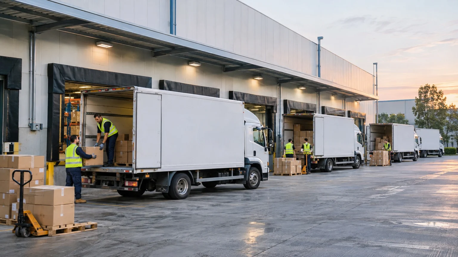
Every morning in front of a distribution center, a line of trucks waits to leave with their loads. There are dozens of stops to make today, and someone has to decide which truck takes which house and in what order. Even for the same parcels going to the same homes, how the routes are drawn makes a big difference in the distance driven, the fuel bill, and the time the driver gets off work.
Put simply, the vehicle routing problem is “the problem of finding the set of routes with the lowest total cost when several vehicles leave a depot, divide up the customers to visit, and return.” It was first introduced in 1959 by George Dantzig and John Ramser as a problem of dispatching trucks to deliver gasoline to filling stations, and today it is the basic calculation behind parcel delivery and distribution logistics.
In this article, we will look in turn at the basic structure of the vehicle routing problem, why the number of possibilities explodes, the many conditions that reality adds, and the ways of finding an answer.
A Calculation That Plans the Routes of Many Trucks at Once
The Basic Structure of the Vehicle Routing Problem
The vehicle routing problem becomes clear once you pin down just a few elements.
(1) The depot and the vehicles
Every vehicle leaves from a single depot, that is, a home base, and returns there after finishing its work. How many vehicles there are and how much each can carry are fixed from the start.
(2) Customers and demand
Every stop has a location and an amount of goods it must receive. Each customer must be served exactly once, and by only one vehicle.
(3) Travel cost
The distance, time, or money needed to travel between two points is worked out in advance. If you find the shortest path on the real road network first, the costs between points can be handled like a single table.
(4) The objective
The most common objective is to reduce total travel cost. In some cases the goal is instead to use as few vehicles as possible, or to divide the workload evenly among the vehicles.
Why the Number of Possibilities Explodes
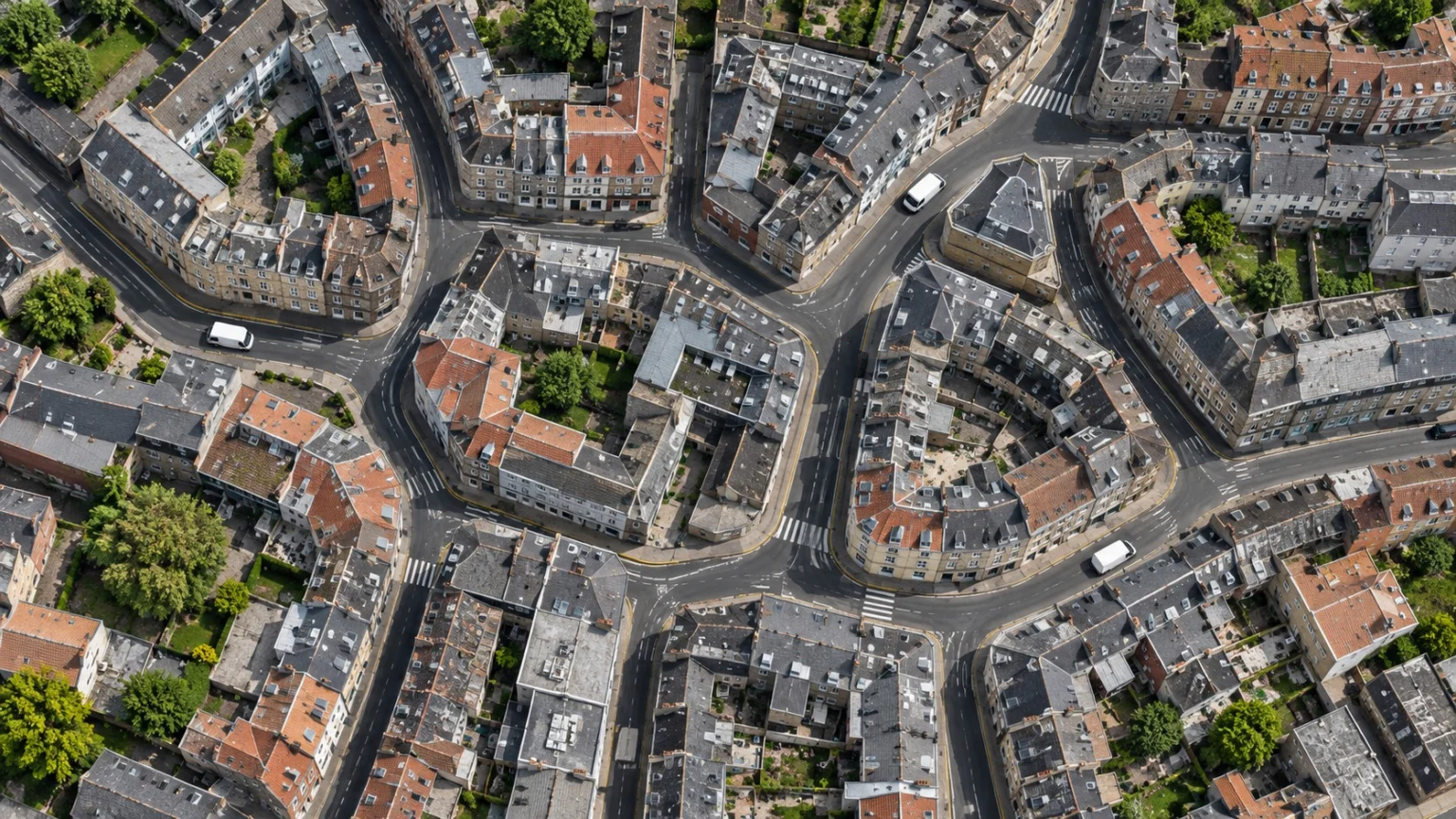
The problem of finding the shortest order for one truck to make a single loop through all the houses is called the Traveling Salesman Problem. The vehicle routing problem extends this to several vehicles, so it is at least that hard.
With 10 places to visit, the order of the stops alone gives about 3.62 million possibilities. With 20 places, that number swells to about 2.43 quintillion. On top of that you have to decide which vehicle serves which customer, so checking every possibility one by one quickly hits a wall.
In mathematics, problems like this are classed as NP-hard. It means the time needed to find an exact answer can grow at an unmanageable pace as the number of customers rises. That is why, in practice, people often choose to find a good enough answer quickly rather than a perfect one.
Conditions That Reality Adds
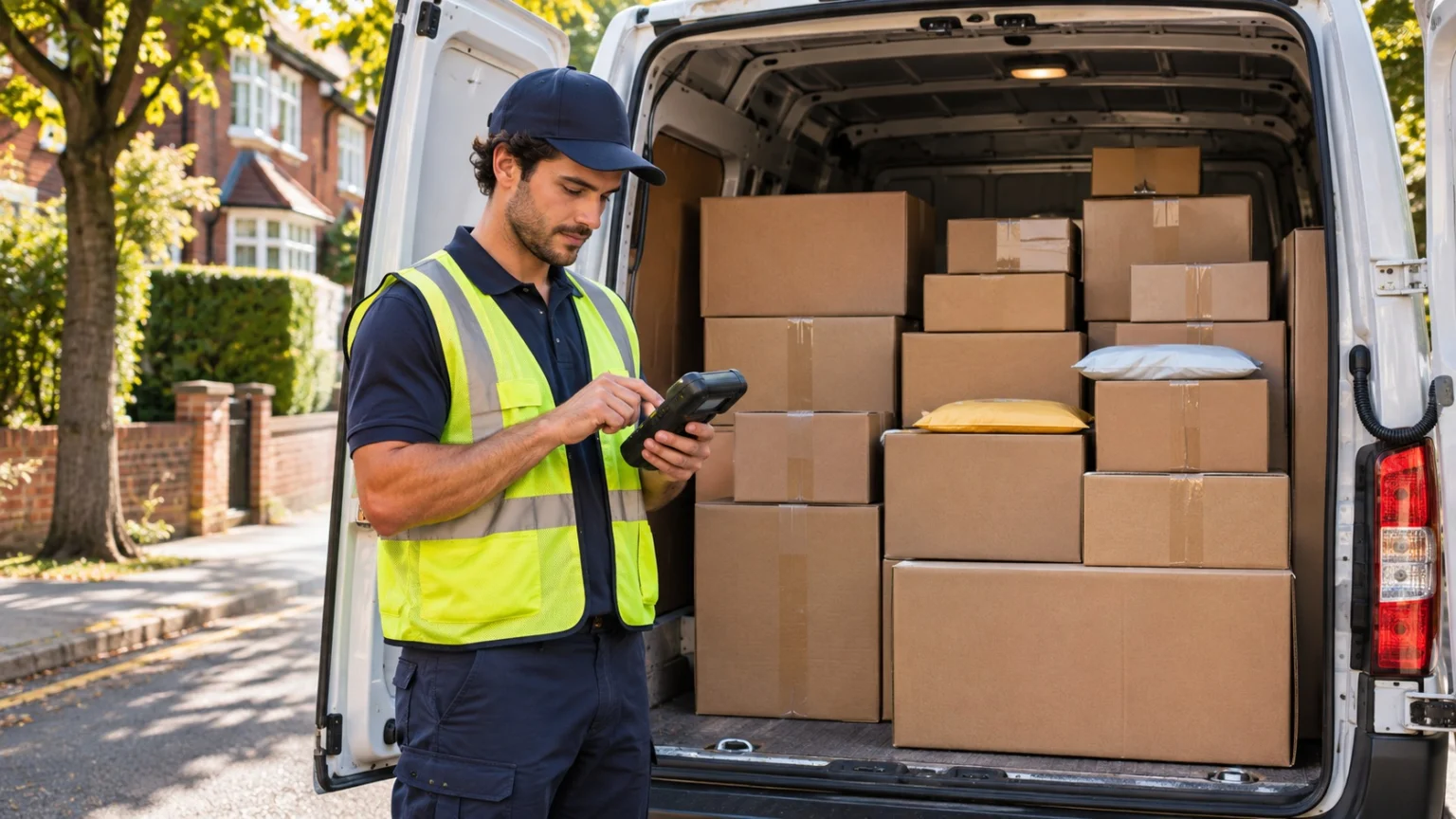
Real delivery work is far more complicated than the textbook problem, and every added condition creates a new variant.
- Capacity constraints (Capacitated Vehicle Routing Problem): each vehicle has a limit on the weight or volume it can carry, so customers must be divided without exceeding it.
- Time window constraints (Vehicle Routing Problem with Time Windows): each customer can receive goods only within a set period, and the vehicle must arrive inside it.
- Pickup and delivery (Vehicle Routing Problem with Pickup and Delivery): goods are loaded at one place and dropped off at another, and both jobs are handled together.
- Multiple depots (Multi-Depot Vehicle Routing Problem): there are several depots that vehicles leave from and return to.
- Electric vehicles (Electric Vehicle Routing Problem): the distance a battery allows and the places to recharge are taken into account too.
Beyond these, many more variants are studied to match the circumstances in the field, such as cases where vehicles do not have to return to the depot, or where they go back and forth to the depot several times a day.
Ways of Finding an Answer

The ways of solving the vehicle routing problem fall broadly into those that seek an exact answer and those that seek a good answer quickly.
Exact Methods
These set the problem up as a mathematical model called integer programming, then cleverly filter out possibilities to find the best answer. The quality of the answer is certain, but computation time grows sharply as customers increase, so they are mostly used for small problems.
The Savings Algorithm
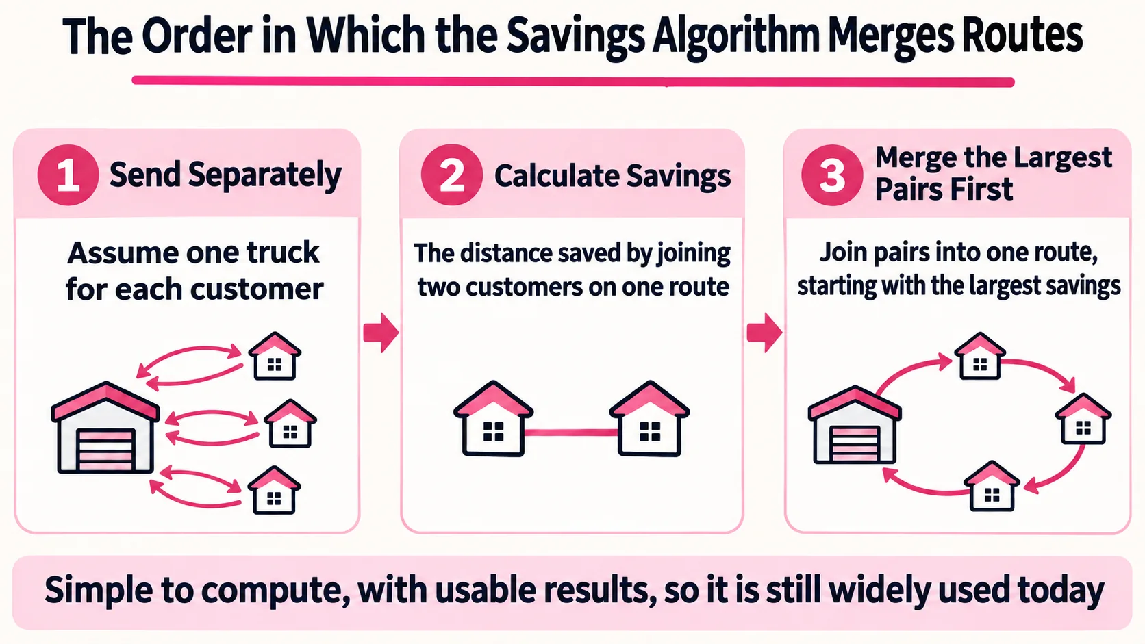
This method was proposed in 1964 by G. Clarke and J. W. Wright. It first assumes that a separate truck is sent to each customer, then merges routes in order, starting with the pair of customers whose joining into one route saves the most distance, that is, the largest savings. It is simple to compute and gives usable results, so it is still widely used today.
Metaheuristics
Methods such as genetic algorithms, tabu search, and simulated annealing improve an initial route bit by bit to find better and better answers. The best recent methods are said to come within about 1 percent of the optimal answer even on problems with hundreds to thousands of stops.
The vehicle routing problem looks like drawing lines on a map, but behind it lies a calculation that tries to cut cost, time, and human labor all at once. That vendors of route-planning software advertise cost savings of 5 to 30 percent shows the power of this calculation.
Constantly reworking routes to carry the same load over a shorter road: that is the first step toward efficient delivery.